Predicting ESG risks with Pytorch, Google Trends and Amazon SageMaker
Introduction
The project deals with a prediction task within finance, and in particular, sustainable investment. Private investors increasingly demand firms that act socially responsible, environmentally friendly and have good governance. The UN and leading asset management firms developed the three pillars of ESG, namely environmental, social and governmental, in a conference in 2005 (International Finance Corporation et al., 2005).
A few years ago investors were willing to accept lower returns for socially responsible investments, but firms with higher ESG scores closed the gap. Auer & Schuhmacher (2016) do not find lower returns of ESG investing compared to a market portfolio. This gives way to an increased demand by investors to invest according the ESG pillars and favor firms that score higher in ESG ratings. FTSE Russell (2018) finds that more than half of global asset owners are currently implementing or evaluating ESG considerations in their investment strategy.
ESG becomes increasingly relevant in today’s investment decisions, especially in the face of global challenges such as climate change, human rights abuse or gender equality. That is why I want to find out more about ESG scores and how they can be predicted for firms using non-primary data from Google Trends.
Problem Statement
ESG investing requires individual investors to be disproportionately well informed. A lot of data about a firm has to be collected, processed and interpreted which leads to a high workload and cognitive strain.
A fundamental problem lies in conflict of interest of the firm to not disclose anything which leads to bad press. Reports on sustainability, corporate social responsibility and even financial reports are often subject to manipulation at worst or overly positive framing at best. It is hard to distinguish between a company that is truly transparent and lives up to its self-defined sustainability principles or just pretends to act accordingly. To break this information asymmetry it often involves third parties, such as investigative journalism, whistle blowing or tight regulation.
Overall ESG scores and ratings can be a starting point for ESG investing and provide a shortcut. Investors rely on different approaches to construct ESG compliant portfolios. One such approach excludes firms that fulfill negative criteria, such as being badly governed, involvement in scandals or even reliance on fossil fuels.
Still, some investors want to be informed in detail, but their hunger for transparency is not met by the firm, which wants to hide and obscure scandals, visible in the media. A firm experiencing a scandal is salient to the public, why it likely appears more frequently in Google searches. Furthermore, providers of publicly available ESG ratings might not update their scores as frequently as professional paid services. Google trends can indicate short-term sentiment against a firm when negative criteria spike in search frequency.
Another factor is about the complexity of ESG ratings. There is no standardized or regulated way to calculate ESG metrics, which leads to multiple methodologies to construct them. Each provider sells their methodology as superior, while details sometimes remain obscure. This is especially the case when sentiment analyses are included which involves intricate data collection, processing and modeling, which is too much to digest for an investor who tries to fully understand how they derive ESG metrics. In contrast to this, relying on Google searches is straightforward to understand and reduces complexity.
Therefore, the project investigates the potential of using Google trends to infer ESG scores and focuses on the main question:
Can Google trends and machine learning inform investors about a firm’s ESG performance?
A more technical version of the problem statement could be: Can machine learning models classify firms in their ESG performance based on Google search frequency?
Main results
The answer the these questions can be summarized in three main results:
- Gathering data through Google trends is time consuming and works without errors with 20 seconds timeout after each keyword query
- Negative keywords for ESG criteria positively correlate with each other and share one underlying latent factor that accounts most for the explained variance
- The neural network predicts slightly better than a random guess, which likely stems from limitations of the data
The analysis concludes with an outlook on follow-up projects. Future work should focus on extensive datasets with features that also include positive screening keywords
Implementation roadmap
To arrive at the results and structure my work, I followed a detailed implementation plan.
- Data collection
- Get tickers from S&P 500 on Wikipedia
- Get main outcome: ESG risk, obtained through the yahooquery Pypi package (accessed with the parameter esg_scores for a ticker)
- Obtain search metrics on ESG related keywords from Google trends through the pytrends Pypi package
- Data processing and feature transformation
- Collapse time dimension of Google trends search index into the following metrics for each keyword, using a defined time span, such as one year
- Average search index across one year
- apply an exponential decay function as a weight, assigning higher weight to the most recent year
- create binary classifier based on median split on ESG score, indicating high and low ESG performers
- Re-shape dataset into wide format, with columns as features and rows as firms
- Split data into a train and test set, convert to .csv and upload to S3
- Descriptive statistics
- List top-5 means of some variables
- Correlation heatmap
- inspect the outcome variables
- Training, validating and testing a model with Sagemaker
- Write scripts for logistic regression benchmark: train.py
- Write scripts for PyTorch neural network: model.py and train.py
- Instantiate estimators with Sagemaker
- Run training job
- Deploy models for testing
- Evaluation and benchmark comparison
- Key metrics for model performance: accuracy, precision and recall
- Possible model adjustment of the neural net when it lacks precision
- Clean up resources
- Delete endpoint
- Remove other resources, such as emptying S3 bucket training jobs, endpoint configurations, notebook instances
Data
The following sections describe how I construct the dataset from scratch. First, Google trends is introduced and how keywords are composed. Second, the Pytrends library is described along with challenges imposed by Google’s unknown rate limits as well as the metric of search interest over time.
Constructing the dataset
Google trends ( https://trends.google.com/trends/?geo=US ) shows search interest for a given keyword within a specified region. As a starting point, I deal with American firms and thus focus on the US using English keywords. The Google trend indicator quantifies the relative search volume of searches between two or more terms.
Relative search volume could be interpreted as search interest and ranges from 0 to 100. To be clear, it lacks a defined measurement unit such as an absolute search count, but relates to all other keywords that were part of the query to Google trends.
A popular procedure to select ESG investments is by checking on whether a firm fulfills defined exclusion criteria, which is termed negative screening. For example, if a firm engages in arms trade, it would be excluded from ESG portfolios. Some other examples are firms linked to corruption, relying on fossil fuels or notorious for avoiding taxes. On the opposite, another ESG investment approach would be positive screening, where a person selects firms since they rely on renewables, promote gender equality or score high in transparency.
I constructed 30 keywords based on negative screening, since issues about a particular firm likely appear in the news and are therefore more salient to the public than a corporate social responsiblity project mentioned in a sustainability report. I chose them in a way to cover a broad range of relevant topics for negative screening and derived them in part from negating UN’s sustainable development goals ( https://www.un.org/sustainabledevelopment/sustainable-development-goals/) . Additionally, I included general keywords that people will search for, when they suspect a firm acting against their morale, such as “firm xy issues” or “firm xy bad”. Keywords like “scandal” or “lawsuit” will possibly cover a lot of specific terminology used by ESG investors for negative screening, but are assumed to be more common among individuals.
The overarching themes within my keywords inlcude ecological impact, gender equality, activities against law, negative news coverage, negative public image and weapons. All in all, I composed 30 keywords to capture a broad range of negative screening criteria and included the following keywords:
'scandal', 'greenwashing', 'corruption', 'fraud', 'bribe', 'tax',
 'forced', 'harassment', 'violation', 'human rights', 'conflict',
 'weapons', 'arms trade', 'pollution', 'CO2', 'emission', 'fossil
 fuel','gender inequality', 'discrimination', 'sexism', 'racist',
 'intransparent', 'data privacy', 'lawsuit', 'unfair', 'bad', 'problem',
 'hate', 'issues', 'controversial'
The topical keywords need to be merged with firm names to end up with keywords that are passed to Google trends. To achieve this, I merge the topic keywords with firm names and get topic-firm pairwise combinations, such as
'scandal 3M ', 'greenwashing 3M ', 'corruption 3M ', 'fraud 3M 'or 'bribe 3M '
Using Pytrends at scale for Google Trends
To access data from Google trends and establish a connection, the project relies on the Pytrends package. Several issues arise from gathering data with Google trends. Firstly, Google trends allows a maximum of five keywords per query. Secondly, a rate limit exists which protects Google’s servers from too many requests. Thirdly, the metric of search interest is scaled based on the search interest of the keyword with the most searches as compared to other keywords. The query limit requires a simple workaround, where I need to batch keywords and subsequently pass each keyword batch to Google trends. With $500$ firms, $30$ keywords and a batch size of $5$, there are $500 \times 30\times \frac{1}{5}=3000$ queries.
The rate limit calls for a timeout. Since Google does not publish information about their search backend due to secutiry reasons, the exact rate limit is unknown. But, query errors lead to missing data entries, which leads to fewer data points to train, validate or test the model. Therefore, I favor a conservative approach, setting the timeout to 20 seconds. The downside of this are runtimes of $3000 \times 20 $ seconds $= 60.000$ seconds $\approx 16.7$ hours. A distinct jupyter notebook that exectutes queries in the background and stores query responses in a csv in case of error response, frees up coding capacity for model setup and avoids data loss caused by rate limits.
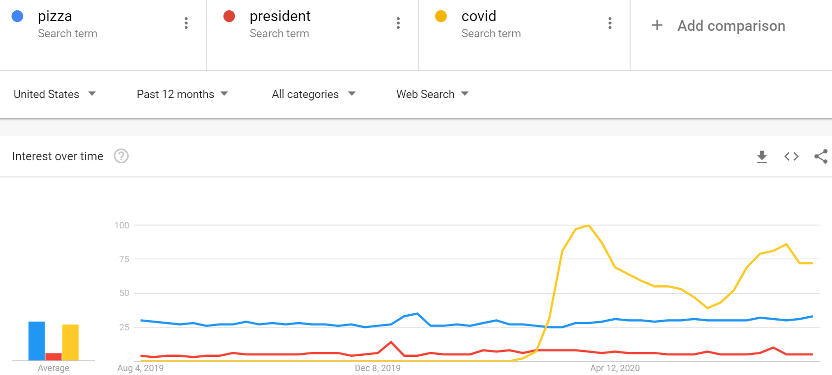
The last challenge with Google trends is the relative search metric. To exemplify this, a query of three words with [‘pizza’, ‘president’, ‘covid’] scales the search interest to the keyword with the most number of searches. The images below illustrate this. It would be a cause of concern when keywords belong to distinct informational sets. Nevertheless, the constructed keywords have the firm name in common, which makes outliers in search interest across queries unlikely since they have the firm name in common. To be concice, I assume that the firm name sufficiently conncets keywords and thereby reduces outliers caused by the relative metric.
Below is the main code snippet, illustrating the timeout function and querying Google trends in a way to not raise any exceptions.
# PYTREND HELPERS
def pytrends_sleep_init(seconds):
    """Timeout for certain seconds and re-initialize pytrends

    Input
        seconds: int with seconds for timeout

    Return
        None

    """
    print("TIMEOUT for {} sec.".format(seconds))
    sleep(seconds)
    pt = TrendReq()


# Define timeout
sec_sleep = 20


# initialize pytrends
pt = TrendReq()

# store DFs for later concat
df_list = []
index_batch_error = []

# create csv to store intermediate results
make_csv(pd.DataFrame(), filename='googletrends.csv', data_dir='data', append=False)

for i, batch in enumerate(keyword_batches):

    # retrieve interest over time
    try:
        # re-init pytrends and wait (sleep/timeout)
        pytrends_sleep_init(sec_sleep)

        # pass keywords to pytrends API
        pt.build_payload(kw_list=batch)
        print("Payload build for {}. batch".format(i))
        df_search_result = pt.interest_over_time()

    except Exception as e:
        print(e)
        print("Query {} of {}".format(i, n_query))
        # store index at which error occurred
        index_batch_error.append(i)

        # re-init pytrends and wait (sleep/timeout)
        pytrends_sleep_init(sec_sleep)

        # retry
        print("RETRY for {}. batch".format(i))
        pt.build_payload(kw_list=batch)
        df_search_result = pt.interest_over_time()

    # check for non-empty df
    if df_search_result.shape[0] != 0:

        # reset index for consistency (to call pd.concat later with empty dfs)
        df_search_result.reset_index(inplace=True)
        df_list.append(df_search_result)

    # no search result for any keyword
    else:
        # create df containing 0s
        df_search_result = pd.DataFrame(np.zeros((261,batch_size)), columns=batch)
        df_list.append(df_search_result)

    make_csv(df_search_result, filename='googletrends.csv', data_dir='data',
             append=True,
            header=True)
Preprocessing and feature engineering
To feed the data into the model, it has to meet certain criteria. A simple data format has rows for individuals and columns for an individual’s characteristics. In this example, it should be a matrix where one row stands for one firm and where columns contain information about the firm.
However, Google trends returns a time-series for each keyword spanning the last five years, reported weekly. This amounts to $260$ ($52$ weeks $\times$ $5$ years $= 260$) entries for each keyword and yields the so-called “long” data format for a given firm, A and 30 search keyword:
| Firm | time | keyword_1 | … | keyword_30 |
|---|---|---|---|---|
| A | 1 | 25 | … | 30 |
| A | 2 | 25 | … | 30 |
| … | … | … | … | … |
| A | 260 | 25 | … | 30 |
Thus, the data needs to be re-shaped into a wide format as previously described. Ideally, re-shaping does not imply information loss. Nevertheless, weekly data might be too granular for the prediction task and likely does not add valuable information as compared to year averages. Thus, taking yearly averages is assumed to have sufficient information about a topic. Peaks in search volume are mirrored by higher year averages instead of week-to-week differences. Averaging by year, adding the time dimension to keywords variables and thereby collapsing the time dimension, yields the wide format. The following table illustrates the desired wide format, which can be fed into the model:
| Firm | keyword_1_t1 | keyword_1_t2 | … | keyword_30_t5 |
|---|---|---|---|---|
| A | 0 | 2 | … | 50 |
| B | 3 | 25 | … | 77 |
| … | … | … | … | … |
| Z | 14 | 60 | … | 42 |

Overview of the final dataset
The dataset is a $N\times(M+1)$ matrix which contains overall $N=305$ rows, $i$, with $M=145$ features, $X_m$, and one outcome variable, $y$. The $145$ features, $X_m$, indicate year-average search interest for a keyword-firm combination at time $t$, which spans five years, indicated by the variable suffixes $0$ to $4$.
The outcome variable, $y$, is a firm’s overall ESG score. Which is later used to construct the binary ESG score high/low variable through a median split. Besides this binary variable, all other metrics count as a ordinal attribute types. They are ordered, while their relative magnitude has no physical meaning. ESG scores rank firms relatively within sector, so that a one point difference for one firm does not mean the same for another. The same holds for relative search interest for a given keyword-firm pair.
Descriptive statistics
Variable means
I focus on the most recent period, corresponding to the time window from today to 1 year ago. The variables have suffix $_4$ and were not downward weighted by the decay function, which means we see the unprocessed metric for search interest. Looking at top-five highest and lowest variable means yields the following tables.
| Variable | 5 highest means |
|---|---|
| tax_4 | 14.731021 |
| bad_4 | 13.299369 |
| problem_4 | 4.437894 |
| issues_4 | 4.334615 |
| fraud_4 | 4.154477 |
| Variable | 5 lowest means |
|---|---|
| harassment_4 | 0.103090 |
| bribe_4 | 0.001955 |
| greenwashing_4 | 0.000000 |
| intransparent_4 | 0.000000 |
| arms trade_4 | 0.000000 |
Correlations
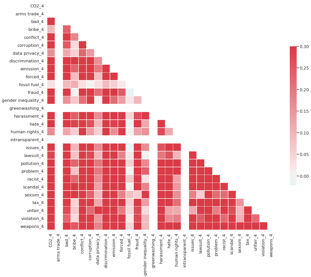
The correlation heatmap depicts a uniform pattern of rather strong positive correlation around .25. Additionally, it makes variables with zero variance and means salient. Normally, we would like to see more intricate correlations and uniform patterns such as these are uncommon. However, this is due to choice of keywords, which all relate to negative criteria within the ESG setting. Since they share this overarching theme, the uniform pattern becomes explainable and motivate other approaches to include more diverse keywords that also include ESG topics of positive screening.
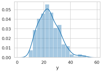
Distribution of the outcome variable
Below is the distribution of ESG scores on which the median split is based. It shows a few outliers to the right, but seems evenly distributed. It shows that a median split is a rather safe clean way to divide the data.
Principle component analysis (PCA)
Explained variance
As an additional part of descriptive statistics, I conduct a principle component analysis (PCA). Plotting explained variance of each component indicates how many latent features are present in the data. Both the scree plot and the table below show a sharp decline of explained variance from the first to the second component, where the latter accounts for less than 1/4 explained variance of the first component. This might hint at a latent factor across multiple features and a larger interdependence among them, as similarly indicated by the correlation pattern.
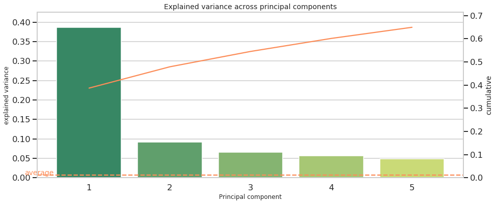
| PC | explained variance | cumulative |
|---|---|---|
| 1 | 0.386840 | 0.386840 |
| 2 | 0.091858 | 0.478698 |
| 3 | 0.066203 | 0.544901 |
| 4 | 0.056188 | 0.601089 |
| 5 | 0.048013 | 0.649102 |
To further pin down the hypothesis about latent factors, factor loadings can be examined. In some cases, factor loadings reveal a common pattern, where in other cases, it cannot be easily interpreted when it does not match into a narrative. Therefore, the next section deals with factor loadings.
Factor loadings
Below is a table showing the top-3 highest and lowest factor loadings for the first principle component.
| PC 1 | lowest factor loadings |
|---|---|
| arms trade_0 | -1.110223e-16 |
| greenwashing_1 | -0.000000e+00 |
| intransparent_4 | -0.000000e+00 |
The lowest coefficients show zero connection to the keywords arms trade, greenwashing and intransparent. Referring to the mean statistics above explains these low values, since these variables do not have any variance, being a constant 0.
| PC1 | highest factor loadings |
|---|---|
| conflict_2 | 0.122832 |
| conflict_0 | 0.121809 |
| conflict_1 | 0.121395 |
| conflict_3 | 0.120161 |
| conflict_4 | 0.119546 |
| weapons_2 | 0.118173 |
| weapons_1 | 0.117959 |
| weapons_3 | 0.117439 |
| weapons_0 | 0.116779 |
| weapons_4 | 0.115938 |
| discrimination_2 | 0.112915 |
| discrimination_0 | 0.112702 |
| discrimination_4 | 0.112656 |
| discrimination_1 | 0.112234 |
| discrimination_3 | 0.112179 |
Inspecting the highest factor loadings uncovers a strong link to keywords of conflict, weapons and discrimination. These factors not only proxy similar firm traits, but are also of similar magnitude, ranging around 0.1. This hints at a strong latent foundation across features, which is by construction from the chosen topics. All ESG topic keywords stem from the idea of negative screening which comprises negative criteria. If there would be a more diverse spectrum of keywords, this likely leads to a less uniform distribution of factor loadings and a less distinct drop of explained variance from one principal component to another. The previous correlation analysis hints at informational uniformity across features, which the PCA confirms. The PCA uncovers that one latent factor accounts for most of the variance, which likely stands for negative associations with a firm. Since the keywords were chosen based on this, it is mostly self-constructed.
Methodology
Benchmark model
Two benchmark classifiers are drawn as comparison to the neural network. The first one is a coin flip and the second one a logistic classifier.
By construction of the outcome variable, its median split serves as naive model, where half of the firms fall into the positive category, even though they perform low on ESG. The naive approach is equivalent to flipping a coin, achieving an accuracy of 50% on average. The second benchmark is a logistic classifier, which is a simple but commonly found classifier.
Neural network with Pytorch in Sagemaker
I implemented the neural network with Pytorch on Amazon Sagemaker, with the necessary scripts train.py, model.py and predict.py in the corresponding pytorch_source folder. Furthermore, a Sagemaker Pytorch estimator object was trained using a 80%/20% train-test split. Thereafter, I deployed the model for testing purposes and generated the predictions on the test set. Additionally, all classification metrics were retrieved. All implementation steps for Pytorch were repeated for the Sklearn logistic classifier, excluding the model.py and predict.pyscripts. For model comparison, the evaluation metrics of both models were merged. As a last step, Sagemaker’s resources were cleaned up, deleting endpoints and data from the S3 bucket.
This is how pytorch instantiated on Sagemaker in detail, specified with 512 hidden dimensions, 40 training epochs and the number of features (145).
from sagemaker.pytorch import PyTorch

# select instance
instance =  'ml.m4.xlarge'

# specify output path in S3
output_path = 's3://{}/{}'.format(bucket, prefix)
print("S3 OUTPUT PATH:\n{}".format(output_path))

# instantiate a pytorch estimator
estimator = PyTorch(entry_point='train.py',
                   source_dir='source_pytorch',
                   role=role,
                   framework_version='1.5.0', #latest version
                   train_instance_count=1,
                   train_instance_type=instance,
                   output_path=output_path,
                   sagemaker_session=sagemaker_session,
                   hyperparameters={
                       'input_features': 145,
                       'hidden_dim': 512,
                       'output_dim': 1,
                       'epochs': 40
                   })

# Train estimator on S3 training data
estimator.fit({'train': input_data})
The logistic classifier was similarly instantiated using a Sklearn estimator object.
Results
Model Performance
The final neural network scores 55.7% accuracy, which is slightly better than chance. The logistic classifier scores 7 percentage points lower with an accuracy of 48.7% being worse than a coin flip. This shows that the neural network performs best given the limitations of the data. With more extensive data, having more features and firms, it is expected to perform even better.
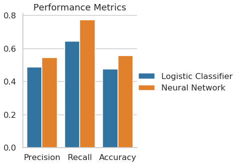
| Model | Precision | Recall | Accuracy |
|---|---|---|---|
| Logistic Classifier | 0.487805 | 0.645161 | 0.475410 |
| Neural Network | 0.545455 | 0.774194 | 0.557377 |
However, it also consumes disproportionately more computational resources than the simple benchmark. It is up to future work, whether this performance advantage grows or shrinks with more extensive data.
The model builds on Pytorch as a neural network. It consists of three fully connected linear layers with a sigmoid function as the output layer. Feedforward behavior is defined by three rectified linear units (relu) as hidden layers, two dropout layers to avoid overfitting, and lastly, the sigmoid output layer. The dimensions for hidden layers were chosen to be particularly high to start of with a rather complex model, which could the be pruned to reduce computational expense.
An observation passes through the network as follows. First, the 145 input features pass the first hidden layer with 512 relu, followed by a 20% dropout layer. Second, the signals proceed to the second hidden layer with $512/2=256$ relus, followed again by an equivalent dropout layer, followed by a third hidden layer, which outputs one dimension. Lastly, the signal enters a sigmoid function to predict an outcome.
Lack of data causes the models to score low in accuracy and related metrics. Robustness checks would be sensible if a model is expected to perform as part of an application. However, at such low accuracy, the largest scope for improvement lies in more and high quality data. A matter of concern is high correlation between features, which can be tackled by adding additional features, that correlate negatively among each other, thereby increasing the chances to add predictive power for ESG scores. One example could be financial data, which could be merged to the existing dataset.
Even though, more extensive data likely contributes to the largest accuracy gains, I outline robustness checks below. I leave their implementation to a future version of this project.
- Model: Change model parameters by increasing the number of hidden layers
- Data: Define ESG top performers as firms that fall into the highest 25 percent of ESG scores instead of a median split.
- Data: use a continuous outcome such as the ESG score instead of a binary target and analyze the model’s prediction error
- Data: drop the time dimension and aggregate across all five years
- Data: Check the influence of the decay function dataset with and without time dimension
Conclusion
To conclude, I conceptualized, developed and implemented a data analysis project from scratch which mainly deals with search frequency of keywords from Google. Major challenges were faced while collecting the data which compromised the extensiveness of the data and depth of model analysis.
The main question: “Can Google trends and machine learning inform investors about a firm’s ESG performance?” can be answered with a cautious ‘yes’. On the one hand, the data lacked observations from firms and additional keywords. On the other hand, there is great potential to re-use procedures to query Google for follow up and an extension of the project.
Appendix
README
I conducted this project as part of the Machine Learning Engineer Nanodegree at Udacity in August 2020.
Python libraries
It relies on the following libraries or services
- Python (3.6)
- Pytorch (1.4.0)
- Amazon Sagemaker
- Pytrends (4.7.3, https://pypi.org/project/pytrends/ )
- Yahooquery (2.2.6, https://pypi.org/project/yahooquery/ )
The data collection script (1_data_collection.ipynb) takes approximately 17 hours due to Google’s rate limit and a timeout function which avoids server errors. It is therefore recommended to load the provided csv data files for replication.
Disclaimer
This project is meant to be a pilot for a more rigorous approach to ESG related metrics. I use it to make the error-prone interaction with Google trends accessible, establish work flows with Amazon Sagemaker and identify strengths and weaknesses of the self-collected data. The highly customized data is the major strength of this project. Once established processes to collect data can be easily extended and generalize to other problems, where custom data yields an advantage.
But it also has its drawbacks regarding extensiveness, quality and high upfront costs. Collecting web data takes disproportionately more time than a ready-to-load dataset which leaves less time to work on equally important aspects, such as feature engineering, data processing, model selection, tuning and testing.
All in all, the project yields amazing opportunities for follow-up work and great potential to generalize its data gathering process to other fields. This prototype holds valuable insights, especially for fields where data is scarce and customized solutions that rely on Google search data is crucial.
At the end of this report, I outline a road map for future work and possible extensions. These can be used to further carve out a data science portfolio and discover pathways to untapped data.
References
Auer, B. R., & Schuhmacher, F. (2016). Do socially (ir) responsible investments pay? New evidence from international ESG data. The Quarterly Review of Economics and Finance, 59, 51-62. Bank of America Research (2020). Accessed 28th July 2020, https://www.merrilledge.com/article/why-esg-matters#:~:text=Why%20ESG%20matters%20%E2%80%94%20Now%20more%20than%20ever&text=A%20new%20BofA%20Global%20Research,over%20companies%20that%20don't .
FTSE Russell (2018). Smart beta: 2018 global survey findings from asset owners. Accessed on 29th July 2020, https://investmentnews.co.nz/wp-content/uploads/Smartbeta18.pdf .
Griggs, D., Stafford-Smith, M., Gaffney, O., Rockström, J., Öhman, M. C., Shyamsundar, P., … & Noble, I. (2013). Sustainable development goals for people and planet. Nature, 495(7441), 305-307.
International Finance Corporation, UN Global Compact, Federal Department of Foreign Affairs Switzerland (2005). Who Cares Wins 2005 Conference Report: Investing for Long-Term Value. Accessed 29th July 2020, https://www.ifc.org/wps/wcm/connect/topics_ext_content/ifc_external_corporate_site/sustainability-at-ifc/publications/publications_report_whocareswins2005__wci__1319576590784 .