Disclaimer
This guide aims to be a great resource for practitioners of causal forest and wants to empower researchers with this awesome method. Whether you are a researcher keen to throw your data on causal forest or just want to have a glance for the next study, this article is for you.
I found myself diving into its source code, published papers on its theory and referring to its algorithm reference. I want to combine all these resources in one articlefor you to save time. Still, you are welcome to do so and dig with references.
But as of today 10th May 2021, this guide is in an early stage. I am grateful for any comments and appreciate your input! If you discover inconsistencies, or have questions, I am happy to discuss them with you and revise the tutorial.
Causal forest gains attention as a powerful tool to add a machine learning perspective to empirical studies. The grf software library in R makes it straightforward and quick to apply. Nevertheless, practitioners that want to go beyond basic understanding and include it in their research face many questions and high upfront costs since it largely differs from traditionally used methods, such as ordinary least squares. This article combines insights on its algorithmic implementation, statistical properties and recommended practices to answer
How does causal forest work and how to apply it?
I synthesize five resources to provide an overview. These are (1) Athey et al. (2019) as the main work on its statistical properties, sometimes called “the GRF paper”, (2) Wager & Athey (2018), which propose preliminary procedures for tree-based treatment estimation and honest trees, (3) Athey & Wager (2019) who apply it to an exemplary dataset, (4) the GRF algorithm reference on Github which describes its algorithm, and lastly, (5) R scripts from the Github repository.
Here, causal forest will be applied to data from an educational randomized intervention on grit by Alan et al. (2019) as a hands-on exercise.
Emphasis is on
- procedures and concepts of causal forest
- understanding model parameters
- how to apply it to data
- interpreting its output
Further posts will follow on heterogeneity analyses, parameter tuning, another proposal for replicable models and how model parameters such as honesty and num.trees, impact model performance and precision.
Prerequisites - Before you start
- For this exercise I use
R 4.0.5andGRF 1.2.0. Ensure to have the same versions to replicate the findings. You can check the version with:R.Version()andpackageVersion("grf"). If you need to update a package, unload them first withunloadNamespace("any_package")and runinstall.packages("any_package") - Data can be downloaded on the Harvard Dataverse https://doi.org/10.7910/DVN/SAVGAL
- Knowledge about tree-based methods. I find these resources useful:
- Data Science Lecture 16 (Protopapas, Rader, Pan, 2016)
- Elements of Statistical Learning, Chapter 9.2 “Tree-based methods” (Hastie et al., 2009)
Causal Forest to estimate treatment effects
Athey et al. modified Random Forest by Breiman et al. (2001) to estimate treatment effects. Furthermore, they derive its asymptotic properties and show that it yields unbiased estimators. I briefly explain Causal Trees as its core component and how they form a Causal Forest to estimate conditional average treatment effects. Ultimately, I outline variable importance as a key metric for heterogeneity analyses and mention parameter tuning to obtain data-driven model specifications.
Assume a binary treatment $W_i \in {0,1}$, randomly assigned to treatment ($W_i=1$) and control group ($W_i=0$). Furthermore, assume unconfoundedness following Rosenbaum et al. (1983), where treatment assignment $W_i$ is independent from potential outcomes $Y_i$, conditional on covariates $X_i$ :
$$ { Y_i^{(0)}, Y_i^{(1)} } \perp \!\! \perp W_i \ | \ X_i $$
How Causal Trees grow - Selecting splits (Training)
To see why Causal Forest enables heterogeneity analyses, it is crucial to know the objectives under which each causal tree grows. A causal tree is equivalent to decision trees in its basic structure:
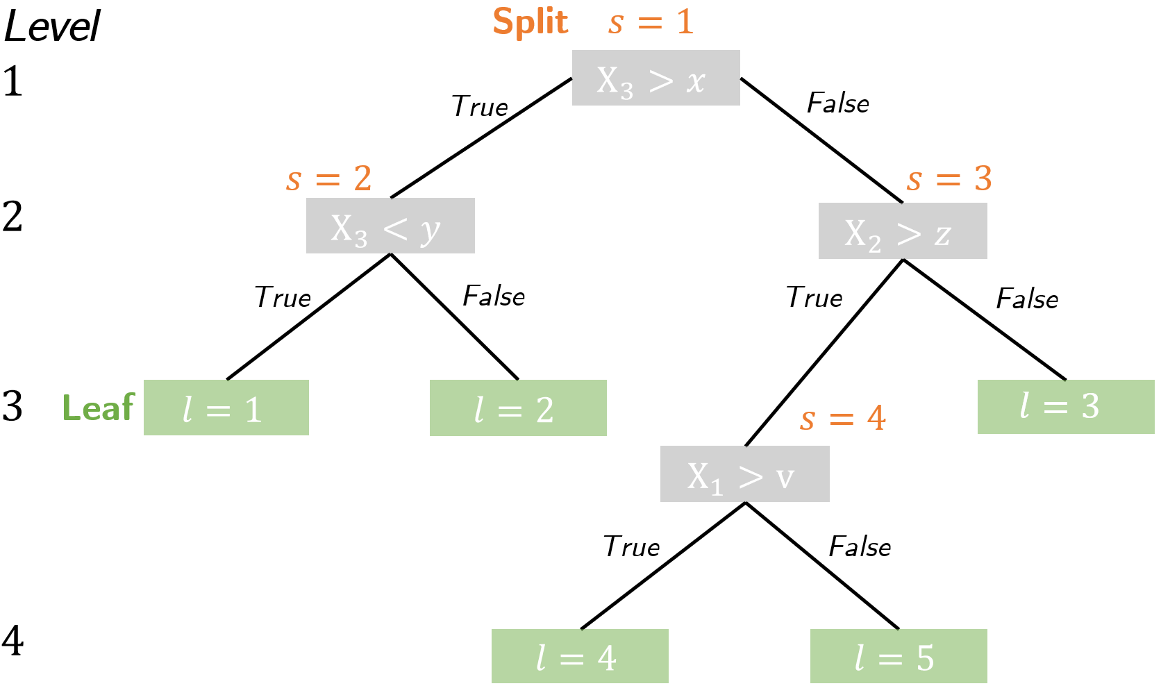
It consists of a root node that branches into child nodes and eventually into terminal nodes, called leafs. At each node, a splitting rule divides observations based on a variable $X_i$ and its split value, such as $x,y,z,v$ in the scheme. Lastly, trees can have different sizes, depending on how many levels it has, with the root node being the first level. Decision trees as in Random Forest differ to Causal Trees in the criteria for a split. The algorithm decides on a split in four recursive steps:
- randomly select a subset of $m$ variables of all $M$ variables that serve as candidates for a split ($m$ is specified with
mtry) - for each of candidate variable, choose a split value $v$, such that it maximizes treatment heterogeneity between resulting child nodes (“split criterion”, see below)
- favor splits with similar numbers of treated and non-treated individuals within a leaf (
stabilize.splits=TRUE) and similar number of individuals across leafs (imbalance.penalty) - account for limiting factors, as given by the minimum number of observations in each leaf (
min.node.size) and maximum imbalance of a split (alpha).
This procedure applies recursively to a random subsample of the data in the training phase until no further splits can be done within a tree when reaching stop criteria as specified in the model.
The exact split criterion from Athey et al. (2019) is defined by
$$ \Delta(C_1, C_2) := \frac{nC_1 nC_2}{n^{2}_{P}} \left( \hat{\theta}_{C_1} (\mathcal{J}) - \hat{\theta}_{C_2}(\mathcal{J}) \right) ^2 $$
where $nC_j$ and $n_P$ are the observation counts for a child node $C_j$ or a parent node $P$ with observations i from the training sample $\mathcal{J}$, i.e. $n_{P,C_j} = | \left( i \in \mathcal{J} : X_i \in {P,C_j} \right) | $.
Honesty (separate training from estimation)
To ensure asymptotically normal and consistent estimates, causal forests use distinct data partitions that make them “honest”. For each tree the data is divided into three parts, as shown in the image below.
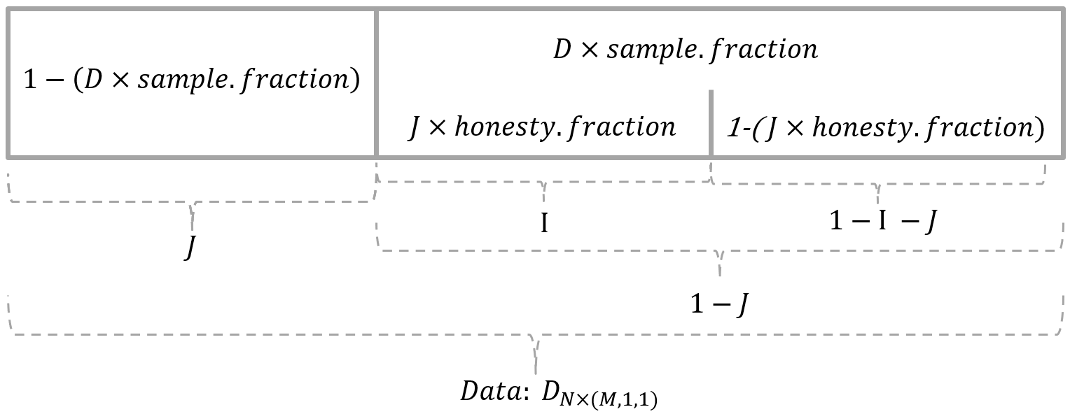
In the training phase, splits are determined with observations from data partition $I \subset J$, whereas outcome prediction is solely done with observations from $(1-I) \subset J$. For prediction, the algorithm distinguishes between estimating an average treatment effect (ATE) and conditional average treatment effects (CATE). ATE can be retrieved with average_treatment_effect([cf object]) and uses outcomes $Y_i$ from $(1-I)$. In contrast, calling predict([cf object]) yields CATE ($\hat{\tau_i}(x)$) which is estimated on “out-of-bag” observations from the partition $(1-J)$. The concept of honesty and this sample split is further described Wager and Athey (2018), section 2.4 and Procedure 1. Double-sample trees.
Estimating conditional average treatment effects (CATE)
Athey et al. (2019) optimized the algorithm in two ways to be computationally feasible while ensuring asymptotic normality and unbiased estimators. First, they replace the exact split criterion with a gradient-based approximation of it (equation (9) instead of (5) in Athey et al. (2019)).
Secondly, they rely on a “forest-based adaptive neighborhood weighting” scheme instead of estimating treatment effects for each leaf of every tree (equation (2) replaced by equation (5) from Wager et al. (2018)). In particular, consider observations from a train and test set, where $i$ belongs to training observations and $x$ to test observations. A Causal Forest consists of trees $t$, where observations fall into its leafs $L$. Each training observation $i$ that falls into the same leaf as test observation $x$ (numerator), receives a positive weight, relative to the size of the leaf (denominator).
$$ \alpha_{ti}(x) = \frac{1({X_i \in L_t(x)})}{|L_t(x)|} $$
These assigned weights for $i$ that fall into the same leafs as test observation $x$ are then averaged across trees, so they sum up to 1: $ \alpha_i(x) = \frac{1}{T} \sum\limits^T_{t=1} \alpha_{ti}(x) $.
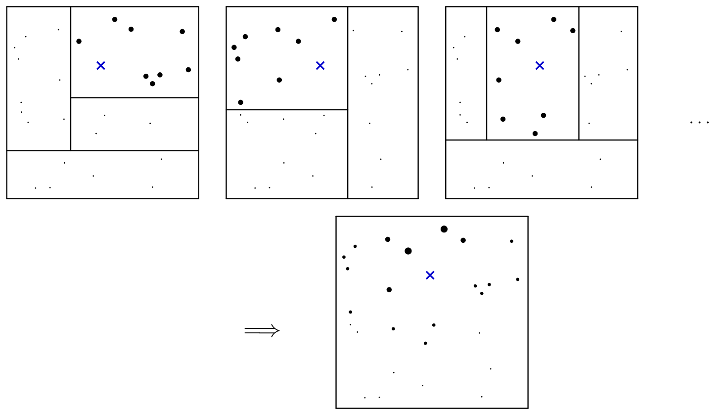
Figure 1 of Athey et al. (2019) illustrates this weighting procedure:
Illustration of the random forest weighting function. The rectangles depticted above correspond to terminal nodes in the dendogram representation of Figure 4. Each tree starts by giving equal (positive) weight to the training examples in the same leaf as our test point x of interest, and zero weight to all the other training examples. Then, the forest averages all these tree-based weightings, and effectively measures how often each training example falls into the same leaf as x.
CATE, $\hat{\tau}_i(x)$, is now based on all outcomes, $Y_j$, weighted by $\alpha_i(x)$. Outcomes of individuals that were already used in the training step are ignored ($D \times sample.fraction$).
Variable Importance
Variable importance indicates how often the algorithm selects a variable to split the sample (A variable that often fulfills the criteria for splits in higher tree levels likely relates to treatment effect heterogeneity, and hence, is deemed more important). Additionally, it is weighted by the level at which the split occurs within a tree, where splits higher up in the tree receive a higher weight.
Hence, variable importance builds on information about the splits, which consists of two parts:
- the count of splits for each variable, called split frequencies, i.e. how often a variable was used to split the sample
- the total number of splits, i.e. how often all variables were used to split the sample in all trees (a total of =
num.trees)
More formally, split frequency, $SF$, as the count of splits for variable $m$ at level $l$ across all trees $t$:
$$SF_{ml} = \sum^T_{t=1} \text{s}_{mlt}$$
where $\text{s}_t = 1$ if variable m used for a split at level l in tree t and $\text{s}_t = 0$ otherwise. This yields a matrix with split counts for each variable and tree levels:
| Var 1 | Var 2 | Var 3 | Var 4 | Var 5 | Var 6 | Var 7 | Var 8 | Var 9 | Row total | |
|---|---|---|---|---|---|---|---|---|---|---|
| Level 1 | 47 | 286 | 614 | 198 | 133 | 224 | 107 | 232 | 157 | 1998 |
| Level 2 | 173 | 531 | 651 | 501 | 209 | 402 | 296 | 560 | 70 | 3393 |
| Level 3 | 267 | 770 | 850 | 508 | 370 | 547 | 417 | 733 | 28 | 4490 |
| Level 4 | 288 | 819 | 949 | 580 | 451 | 590 | 474 | 843 | 7 | 5001 |
Next, each split count is divided by the total number of splits at that level (= row total), which leads to the relative split frequency RSF:
$$ RSF_{ml} = \frac{SF_{ml}}{\sum\limits_{m=1}^M SF_{ml}} $$
Further, a weight is introduced that exponentially favors higher tree levels: $w_l = l^{-2}$. Lastly, apply the weights, $RSF_{ml} \times w_l$, and divide this by the weights’ total, $\sum\limits^L_{l=1} w_l$ to get rid of the level dimension and obtain variable importance:
$$ VI_m=\frac{\sum\limits^L_{l=1} RSF_{ml} \cdot {w_l}}{\sum\limits^L_{l=1} w_l} $$
Case study: A randomized educational study on grit
Study Design
Treatment group (TG): Additional program in elementary and post-elementary schools that features a tailored curriculum for 12 weeks to promote gritty behavior among pupils. To achieve this, teachers inform about (i) growth mindset (“plasticity of the brain against notion of innate ability”), (ii) the role of effort to enhance skills and achieve goals, (iii) failure coping strategies, and (iv) goal setting. Videos, mini case studies, stories and artworks of famous individuals highlight the importance of grit and perseverance from multiple perspectives.
Treatment is randomly assigned across 16 schools (8 treatment + 8 control schools, 1499 pupils of 42 classrooms, where 1360 (91%) were present and consented). Treated schools solely received the grit curriculum. The sample of this intervention is Sample 2 and resolved some design issues of a first intervention, stored in Sample 1. Sample 2’s baseline information was collected in spring 2015, implemented in fall 2015 and tested in January 2016 shortly after the curriculum. Also long-term follow-up was done in June 2017, when students advanced to 5th grade, circa 1.5 years after the intervention (60% could be tracked). The follow-up pupils had slightly different verbal scores at baseline compared to the original intervention sample.
Control group (CG): Several placebo treatments were in place for the control group, including projects on environment sensitivity, health and hygiene.
Data
Outcomes were derived from two incentivized experimental tasks about grit. The first showed a grid with numbers and thed pupils had to find number pairs adding up to 100. Rewards depend on a minimum score (performance target), which was 3 pairs per 1.5 minutes. Before each round, the children decided between a difficult grid and get (i) four gifts or a simpler grid to get (ii) one gift in case of success. Experimenters give feedback after each round if they succeeded or failed to meet the target. Students decided between (i) and (ii) except for the first round, where they got randomly either (i) or (ii) to get a subsample free of selection into the tasks. The following table gives an overview of relevant covariates that are later assigned to causal_forest().
| Variable categories | |
|---|---|
| Demographics | gender, age, teacher estimated socioeconomic status |
| Cognitive skills | Ravens matrices |
| Academic performance | teacher estimated academic success, grades and standardized tests in mathematics and Turkish |
| Risk tolerance | risk allocation task |
| Beliefs (survey) | malleability of skills, attitudes and behavior towards grit and perseverance |
Data Preparation
The quality and preparation of collected data determines the informative value of a study. With many missing entries, researchers have to drop substantial amounts of observations, if they rely on methods requiring data without gaps, such as ordinary least squares (OLS). Alan et al. deal with missings using the simple approach of replacing missings with the average across all other non-missings of each variable. For the analysis here, I focus on the outcome where pupils choose the difficult in all five rounds. The data preparation can be summarized with the following code. Note, that I drop all missings of the outcome $Y (alldiff)$ and replace all missings in $X$ with their average.
df_nomiss <- df %>%
	drop_na(alldiff) %>%
	mutate_at(vars(-alldiff),~ifelse(is.na(.), 0, .))
In contrast, tree-based methods like Random Forest can handle missing data. Causal Forest has been recently extended to handle missing data in the upcoming release of Version 1.1.0. However, right now we have to replace missings as done by the authors using mean imputation . This approach reduces data variability and may introduce biases such as underestimating variance, and thereby, leading to more precise estimates than actually observed. To check for robustness, I replicate their main results (Table III - Treatment effect of choice of difficult task) with and without mean imputation. The results indicate no substantial impact on standard errors through mean imputation.
Replicate results with Ordinary Least Squares (OLS)
Before going further, I want to verify data loading and preparation. If estimates are within ballpark of Alan et al.s’, I can be confident to obtain valid estimates with Causal Forest later on. To keep it simple, I choose ordinary least squares instead of logit as in their paper, since the latter needs some workarounds for obtaining average marginal effects with clustered standard errors (a combination of the mfx and miceadds package solves this). Therefore, estimates should differ slightly from theirs, but would have similar magnitudes.
Below you find the estimated treatment treatment effects employing ordinary least squares.
| Difficult round 1 | Difficult round 2 | Difficult round 3 | Difficult round 4 | Difficult round 5 | |
|---|---|---|---|---|---|
| Est. treatment effect | 0.10 | 0.16 | 0.16 | 0.16 | 0.14 |
| Std. Error | 0.04 | 0.04 | 0.04 | 0.05 | 0.04 |
| Intercept | 0.57 | 0.32 | 0.15 | 0.06 | 0.05 |
| N | 1354 | 1351 | 1351 | 1350 | 1354 |
The estimates correspond to those in Table A.8 of their online appendix (Alan et al., 2019) and differ slightly from those in Table III. This is reassuring for the steps so far and avoids any issues arising from coarse errors in variable coding. The next section guides through a hands-on example of applying causal forest to the data.
Apply Causal Forest to the data
Assign data
Data provided to the causal_forest function has to have a certain format. First of all, the full dataset is divided into covariates $X$, treatment assignment $W$ and outcome $Y$. The latter two, $W$ and $Y$ have to be a numeric vector, where $W$ can be either $0$ or $1$. The covariate matrix, $X$, can include several variable types, such as categorical, continuous or binary variables. Additionally, it can contain missing values with a caveat for categorical values, that might be hand-coded NA values a new factor (see
#632
,
#475
). Beyond this, clusters can be assigned to obtain clustered standard errors for the estimates.
The following shows how the data parts can be assigned
#covariates (X), outcome (Y), treatment assignment (W) and cluster (cluster)
X <- df_nomiss %>%
	select(male,task_ability,raven,grit_survey1,belief_survey1,
		mathscore1,verbalscore1,risk,inconsistent)
Y <- df_nomiss$alldiff
W <- df_nomiss$grit
cluster <- df_nomiss$schoolid
Parameters for the causal_forest() function
The main function to build a model is causal_forest(), which takes several arguments to specify its parameters. The table below gives an overview of the most important arguments to control the model:
| Parameter | controls |
|---|---|
| num.trees | number of trees grown in the forest more trees increases prediction accuracy, default is 2000 |
| sample.fraction | Share of the data used to train a tree (determine splits) higher fraction assigns more observations to training (within bag) |
| honesty | enable honesty (TRUE, FALSE), where the training sample (data x sample.fraction) is further split to have one sample |
| honesty.fraction | Subsample (= honesty.fraction x (data x sample.fraction)) that is used to choose splits for a tree. Increasing honesty.fraction assigns more data to the task of finding splits. |
| honesty.prune.leaves | whether or not leaves will be removed that are empty when the data from the honesty sample is applied to a tree |
| mtry | Number of variables from covariates (X) that are candidates for a split. When mtry = Number of variables, all variables are tested for a given split |
| min.node.size | minimum number of treated and control group observations for a leaf node. Increasing min.node.size likely leads to fewer splits since child nodes have to meet a stricter condition. A node must contain at least min.node.size treated samples (W=1), and also at least that many control samples (W=0). |
| alpha | the maximum imbalance of a split relative to the size of the parent node. Causal forests rely on a measure that tries to capture ‘information content’ $IC_N$ of a node $N$: $IC_N = \sum\limits_{i \in N} (W_i - \bar{W})^2$. Each child node, $C_{j \in {1,2}}$ has to fulfill $IC(C_j) \geq \alpha \cdot IC(N_{parent}) $ |
| imbalance.penalty | the imbalance of a split between resulting child nodes. Observation count for each child node has to be greater than that of (parent node* alpha). |
| ci.group.size | To calculate confidence intervals, minimum = 2 |
| stabilize.splits | Whether or not the treatment should be taken into account when determining splits |
As the table shows, there are many ways to specify a model through these parameters. Choosing default parameters may not yield the most optimal model, but is a shortcut to spare computing time and obtain a trained forest right away. Another option is to rely on causal forest’s internal parameter tuning that approximates optimal parameters through cross-validation. Even though it is computationally more expensive, approximate optimal values for min.node.size, sample.fraction, mtry, honesty.fraction and honesty.prune.leaves, alpha and imbalance.penalty decreases bias and is easily available by setting tune.parameters='all' in the function. The section in the appendix describes the procedure in more detail.
Nevertheless, parameter tuning throws an error that says instructs to increase the number of trained trees (tune.num.trees) within cross-validation. However, values of up to 50000 could not avoid the error while runtime of the algorithm substantially increased to several minutes. Thus, default model parameters are used.
Applying CF to the data
Orthogonalization. Before assigning the data to causal_forest(), Athey et al. (2019) recommend to fit separate regression trees to estimate $\hat{Y}_i$ and $\hat{W}_i$. Even though, the CF algorithm would do this by default when neither Y.hat nor W.hat are assigned, calling regression_forest() separately sets num.trees=2000 instead of 500 with CF’s default parameters. It ensures more precise estimates for treatment propensity and marginal outcomes to compute residual treatment and outcome.
seed <- 42
set.seed(seed)
Y.hat <- regression_forest(X=X, Y=Y, seed=seed, clusters=cluster)$predictions
W.hat <- regression_forest(X=X, Y=W, seed=seed, clusters=cluster)$predictions
Thereafter, a CF with default parameters is initialized. How to retrieve and interpret these default parameters is explained in the following.
set.seed(seed)
cf_default <- causal_forest(X=X, Y=Y, W=W,
	Y.hat=Y.hat,
	W.hat=W.hat,
	clusters=cluster,
	seed=seed)
Default parameters.
To inspect the model’s characteristics, names(cf_default) lists callable objects.
> names(cf_default)
 [1] "_ci_group_size"           "_num_variables"
 [3] "_num_trees"               "_root_nodes"
 [5] "_child_nodes"             "_leaf_samples"
 [7] "_split_vars"              "_split_values"
 [9] "_drawn_samples"           "_send_missing_left"
[11] "_pv_values"               "_pv_num_types"
[13] "predictions"              "variance.estimates"
[15] "debiased.error"           "excess.error"
[17] "ci.group.size"            "X.orig"
[19] "Y.orig"                   "W.orig"
[21] "Y.hat"                    "W.hat"
[23] "clusters"                 "equalize.cluster.weights"
[25] "tunable.params"           "has.missing.values"
For example, $tunable.params shows the default parameters that would normally be tuned.
cf_default$tunable.params %>% as.data.frame %>%
	rownames_to_column %>%
   	gather(var, value, -rowname) %>%
   	pivot_wider(names_from=rowname, values_from=value)

1 sample.fraction       0.5
2 mtry                  9
3 min.node.size         5
4 honesty.fraction      0.5
5 honesty.prune.leaves  1
6 alpha                 0.05
7 imbalance.penalty     0
To get a feeling for the model specification, I explain the parameters. 25% of the data was sampled to choose splits (sample.fraction$\times$honesty.fraction, $=J$ in the figure above), 25% was used for estimating treatment effects and the remaining 50% held out for out-of-bag prediction. All 9 variables were considered as candidates for a split (mtry). Splits are discarded where leaves contain less than 5 treated or less than 5 non-treated individuals (min.node.size). Honesty will also discard splits, when no observations of the honesty sample (sample.fraction $\times (1-$ honesty.fraction$)$) fall into a leaf. Furthermore, alpha discards splits that likely have nodes with low information content, as approximated by the function $IC_N =\sum\limits_{i \in N} (W_i - \bar{W})^2$, where $N$ is a node. Any child node, $C_{j\in {1,2}}$, must fulfill $IC_{C_j} \geq \alpha * IC_{parent}$. Lastly, imbalance.penalty does not apply, which would favor splits with balanced count of treated and control observation.
I hope you enjoyed the guide so far! Corona-life is keeping me somehow busy and further parts of the tutorial are soon completed and reviewed. If you discover any inconsistencies in my description and coding of the method, I appreciate your feedback. Just hit me on philippschmalen@gmail.com .
References
Alan, S., Boneva, T., & Ertac, S. (2019). Ever failed, try again, succeed better: Results from a randomized educational intervention on grit. The Quarterly Journal of Economics, 134(3), 1121-1162.
Alan, S., Boneva, T., Ertac, S. (2019). “Replication Data for: ‘Ever Failed, Try Again, Succeed Better: Results from a Randomized Educational Intervention on Grit’”. https://doi.org/10.7910/DVN/SAVGAL . Harvard Dataverse, V1, UNF:6:d2Hfm4IAxljvu95OYqXGOQ== [fileUNF].
Alan, S., Boneva, T., Ertac, S. (2019). “Online Appendix Ever Failed, Try Again, Succeed Better: Results from a Randomized Educational Intervention on Grit”, https://www.edworkingpapers.com/sites/default/files/Online%20Appendix.pdf .
Athey, S., Tibshirani, J., & Wager, S. (2019). Generalized random forests. The Annals of Statistics, 47(2), 1148-1178.
Athey, S., & Wager, S. (2019). Estimating treatment effects with causal forests: An application. arXiv preprint arXiv:1902.07409.
Breiman, L. (2001). Random forests. Machine learning, 45(1), 5-32.
Hastie, T., Tibshirani, R., & Friedman, J. (2009). The elements of statistical learning: data mining, inference, and prediction. Springer Science & Business Media.
Rosenbaum, P. R., & Rubin, D. B. (1983). The central role of the propensity score in observational studies for causal effects. Biometrika, 70(1), 41-55.
Wager, S., & Athey, S. (2018). Estimation and inference of heterogeneous treatment effects using random forests. Journal of the American Statistical Association, 113(523), 1228-1242.
GRF-Labs (2020). The GRF Algorithm. https://github.com/grf-labs/grf/blob/master/REFERENCE.md .
Appendix
Orthogonalization
Causal forest assumes that treatment assignment is independent from potential outcomes conditional on $X$. The feature space $\mathbb{X}$ however contains parts related to estimated treatment effects and parts related to treatment propensities. To shift splits towards estimating treatment effects instead of propensities, orthogonalization employs regression forests to estimate (i) treatment propensities and (ii) marginal outcomes which is used as input to grow a causal forest. Estimates of treatment propensities, $ e(x)=E[W|X=x] $, and marginal outcomes, $m(x) = E[Y|X=x]$, yield residual treatments $W-e(x)$ and outcomes $Y-m(x)$. In that way, causal trees solely split on the parts of the variation that contain information on potential treatment effects.
Model error measures
Debiased error: Estimates of the ‘R-Loss’ criterion which relates to the mean-squared error (infeasible). It assumes an infinite number of trees. Therefore, it is complemented by the excess error estimate which captures model induced estimate variance.
Excess error: Jackknife estimates of the Monte-carlo error which relates to estimate variance induced by the trees themselves. The error decreases with more trees and becomes negligible with large forests. To test this, grow forests with different sizes and observe their excess error. The sum of these errors yields the overall error of the forest.
Finding model parameters with parameter tuning
Another feature included for Causal Forest is its automated search for suitable model parameters. The procedure determines close-to optimal parameters for the provided data with cross-validation. However, instead of relying on precise error measures, they are approximated to trade off complexity with lower computational expenses. To enable this for all tunable parameters, set causal_forest(...parameter.tuning='all') and the algorithm looks for determines values for: min.node.size, sample.fraction, mtry, honesty.fraction and honesty.prune.leaves, alpha and imbalance.penalty.
The procedure can be tweaked changing the default values for tune.num.reps, tune.num.trees and tune.num.draws. tune.num.reps is the number of distinct parameter sets that are tested in a mini-forest containing tune.num.trees trees, to obtain a debiased error estimate. Lastly, these error estimates yield a smoothing function to predict the error for another randomly drawn distinct set of tune.num.draws parameters. Those parameter sets that minimize the predicted error are considered optimal.
Variance across Causal Forests
The algorithm selects splits that maximize any given differences in estimated treatment effects between child nodes. However, these differences could be almost negligible and a high variable importance does not necessarily imply heterogeneity across treatment. It solely means that the algorithm selected variables which are more associated with any existing treatment effect heterogeneity than others. Additionally, low heterogeneity could imply that variable importances vary across a set of differently seeded Causal Forests. In that case, slightly varying, random initializations can tip the scales for variable selection and cause different splits. Therefore, it makes sense to explore treatment heterogeneity visually by plotting CATE against values of $X_i$
Especially for lower sample sizes, model parameter have a larger impact on variable importance. Even though, variable importance does not have to be a precise measure, it would be great to obtain robust coefficients.
One way to ensure variable importance for every variable is to force the algorithm to try all variables for each candidate split. mtry is the parameter that controls the number of tried variables and defaults to $\sqrt(M) + 20$ Hold the mtry parameter constant and insert the maximum number, corresponding to the total number of variables.
Remarks on Study Design
- The authors conducted two interventions on grit and patience. Therefore, the dataset contains a “sample” variable to indicate sample 1 or 2. The first sample can be disregarded due to design issues.
- Teachers willing to participate were randomly assigned to TG or CG. Due to this selection into the study, average treatment effect on the treated is observed (ATT). However, since a high share of 80% teachers were willing to participate, the authors conjecture strong external validity. But what are the assumptions and how does it relate to ATE again? This post explains it in brief.
- teachers of the TG attended a one-day training seminar to present materials and suggested classroom activities. Pedagogical guidelines focused on task effort and process instead of outcome-based feedback: Praising effort, rewarding perseverant behavior and favor positive attitudes towards learning.
- verbal and math scores were measured before and after treatment
- data was collected in two classroom visits each a week apart
Results without mean imputation
I was curious, in which way the mean imputation shaped the results. Therefore, I rerun the estimation without mean imputation and obtain:
| Difficult round 1 | Difficult round 2 | Difficult round 3 | Difficult round 4 | Difficult round 5 | |
|---|---|---|---|---|---|
| Est. treatment effect | 0.10 | 0.18 | 0.19 | 0.18 | 0.16 |
| Std. Error | 0.05 | 0.04 | 0.04 | 0.05 | 0.04 |
| Intercept | 0.55 | 0.35 | 0.17 | 0.09 | 0.06 |
| N | 1058 | 1058 | 1056 | 1056 | 1057 |
Mean imputation often leads to more precise estimates and could remove selection issues, when missing values occur in patterns across individuals. Nevertheless, the above table indicates robust estimates in both dimensions with coefficients differing slightly. It looks as if the mean imputation neither changed standard errors nor treatment estimates. Additionally, the estimation method with OLS did not impact coefficients compared to logit as used in the study.
Replicate results with CF (Alan et al., Table 3)
Loop to train 5 causal forests on 5 outcomes (choicer1-5) in the following steps: (i) drop missings for each outcome Y (choicer1-5), (ii) Select and assign X, Y, W and cluster, (iii) train CF model on that data.
	cf_choicer <- lapply(paste0("choicer", 1:5), function(x){

	# (i) Remove missings in Y (while keeping missings in X)
		df_nomiss <- df %>% drop_na(x)

	# (ii) Assign covariates (X), outcome (Y), treatment (W) and cluster
		X <- df_nomiss %>%
			select(male,task_ability,raven,grit_survey1,belief_survey1,mathscore1,
				verbalscore1,risk,inconsistent)
		Y <- df_nomiss[,x] %>% pull #convert to vector with pull()
		W <- df_nomiss$grit
		cluster <- df_nomiss$schoolid

	# (iii) Train CF
		set.seed(seed)
		causal_forest(X=X, Y=Y, W=W, clusters=cluster, seed=seed)
	})

	# Store estimated average treatment effects (ATE)
	cf_ate <- sapply(cf_choicer, function(x){
		average_treatment_effect(x)
})


# Results table
cf_ate %>%
	`colnames<-`(sapply(1:5, function(i) paste("Difficult Round",i))) %>%
	`rownames<-`(c("Est. treatment effect", "Std. Error")) %>%
	rbind(N=sapply(cf_choicer, function(x) nrow(x$X.orig))) %>%
	kable(format="markdown", digits=2)
| Difficult Round 1 | Difficult Round 2 | Difficult Round 3 | Difficult Round 4 | Difficult Round 5 | |
|---|---|---|---|---|---|
| Est. treatment effect | 0.11 | 0.18 | 0.16 | 0.17 | 0.15 |
| Std. Error | 0.05 | 0.05 | 0.06 | 0.07 | 0.06 |
| N | 1354 | 1351 | 1351 | 1350 | 1354 |
The estimated average treatment effects resemble those before obtained with OLS. Standard errors tend to be slightly higher possibly induced by the method and not having imputed.